Logistic Regression
In this section we’ll learn our first classification model class: logistic regression. Our approach will be to “invent” logistic regression for ourselves.
Here’s how we’ll do that:
- Introduce 0/1 classification loss and the risk expression under this loss
- See that we minimise risk under 0/1 loss by choosing the class with largest posterior probability
- Derive the logistic function as a way to model the log probability ratio between two classes
- Derive expressions for log likelihood, surrogate loss, and the gradient-based learning rule
- Generalize logistic regression to multi-class scenarios using the softmax function
0/1 Loss & Risk
0/1 loss is exactly what it sounds like: if we predict the correct class, we suffer no loss, and if we’re wrong, we suffer loss equal 1. Formally:
Notation
- l refers to loss
- h refers to our decision rule, it is a function of observation x
- y refers to the true label for observation x
The expression for the risk of 0/1 loss given a joint probability distribution and a classifier h(x) is:
Above we see that it in order to choose h to minimise R(h), it suffices to choose h which minimises R(h|x) for each x. For a given x:
In words, the conditional risk of 0/1 loss is equal to the probability that your prediction h(x) is wrong. It’s now clear that the way to minimise R(h|x), and thus R(h), is by predicting for each x the class c with the largest posterior p(y=c|x). Formally, our optimal classifier \(h^*\) is given by:
We can express \(h^*\) as a “decision rule” in terms of probability ratios:
Logistic Regression as modelling posteriors
Let us now consider the binary classification scenario. Our work above tells us that the optimal classifier is described as follows:
What we want now is to model the log probability ratio above using a linear function of x:
We can rearrange the equation to get an expression for the posterior:
Notice that, as we’d expect, if \(w \cdot x = 0\), then \(p(y=1|x)=\frac{1}{2}\). That is, if we’re on the decision boundary, then both classes are equally likely.
Negative Log Likelihood Loss
We now turn to the problem of finding “good” w. Since the true joint probability distribution is not known, we cannot directly minimise risk. Instead, we do the next best thing: empricial risk minimisation - that is, we minimise the loss on some training dataset. Suppose we have been given a labeled dataset with N examples.
Notation
- X is the N-by-d matrix of training observations
- y is the N-dim vector of training labels
- w is the d-dim vector of weights
- \(\sigma (z)=\frac{1}{1+exp[-z]}\) denotes the logistic function
It is computationally infeasible to directly minimise 0/1 loss so we instead employ a surrogate loss: negative log likelihood loss (i.e., we want to maximise the likelihood of the training examples). Negative log likelihood loss is given by:
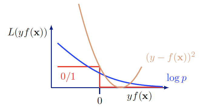
Comparison of the surrogate loss, the original loss, and square error loss (Shakhnarovich, Slide 7, 2018)
Notice that although the expression looks complicated, it’s actually quite simple. For each training example, we want to add the log likelihood of the label \(y_i\) given the observation \(x_i\). The expressions \(y_i\) and \((1-y_i)\) effectively act as if statements that respectively say “if \(y_i = 1\), add \(log p(y_i=1|x_i)\)” and “if \(y_i = 0\), add \(log p(y_i=0|x)\).”
Now that we have this surrogate loss in place, we can derive a gradient-based learning rule for \(w\). (After first doing the scalar partial derivative,) we get (the update is for a single training example):
This learning rule has a nice, intuitive, geometric interpretation. Notice that geometrically, \(w\) represents the normal vector of the decision boundary (in the direction of training examples with \(y_i = 1\)).
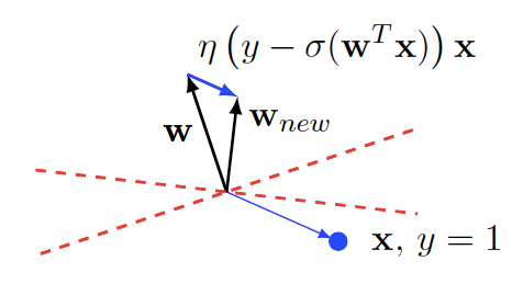
(Shakhnarovich, Slide 7, 2018)
Suppose we’re doing an update based on a single training example \(x_i\) with \(y_i=1\). So the update equation is given by \(w^{t+1} = w^{t} + [1-\sigma(w\cdot x_i)]x_i\). Since \(0 < \sigma(w\cdot x_i) < 1\), the above update always adds a scaled version of \(x_i\) to \(w\). This has the effect of “pulling” \(w\) towards \(x_i\) by some force. The magnitude of the force depends on how well the classifier currently classifies \(x_i\). Consider the two extremes. If our classifier is doing very well, that is \(\sigma(w\cdot x_i)\) is close to 1, \(x_i\) hardly pulls on \(w\). If our classifier is doing very poorly, that is \(\sigma(w\cdot x_i)\) is close to 0, \(x_i\) pulls very hard on \(w\). Updates based on training examples with with \(y_i = 0\) “push” \(w\) instead of pulling it. Quick sanity check: how will the magnitude of the push depend on \(\sigma(w\cdot x_i)\) when \(y_i = 0\)?
The net effect of all this pushing and pulling is that \(w\) will roughly point in the direction towards all the training examples with label \(y_i=1\) and away from all the training examples with label \(y_i=0\).
Generalizing to multi-class with softmax
Notice that logistic regression only works in the binary classification case. But we can easily generalize to the multi-class scenario using the softmax distribution.
Again, we use the negative log likelihood loss to get a learning rule.
Notation
\(\delta_{c y_i}=1\) if \(c = y_i\), else \(\delta_{c y_i}=0\) (Kronecker-Delta)
The geometric intuition we have for the binary class case still applies here in the multi-class case; \(w_c\) is “pulled” in by training examples with \(y_i=c\) and “pushed” away by all other training examples.